aleatory.processes.BrownianMotion#
- class aleatory.processes.BrownianMotion(drift=0.0, scale=1.0, initial=0.0, T=1.0, rng=None)[source]#
Brownian Motion#
A one-dimensional standard Brownian motion object.
Notes#
A standard Brownian motion \(\{W_t : t \geq 0\}\) is defined by the following properties:
Starts at zero, i.e. \(W(0) = 0\)
Independent increments
\(W(t) - W(s)\) follows a Gaussian distribution \(N(0, t-s)\)
Almost surely continuous
A more general version of a Brownian motion, is the Arithmetic Brownian Motion which is defined by the following SDE
\[dX_t = \mu dt + \sigma dW_t \ \ \ \ t\in (0,T]\]with initial condition \(X_0 = x_0\in\mathbb{R}\), where
\(\mu\) is the drift
\(\sigma>0\) is the volatility
\(W_t\) is a standard Brownian Motion
Clearly, the solution to this equation can be written as
\[X_t = x_0 + \mu t + \sigma W_t \ \ \ \ t \in [0,T]\]and each \(X_t \sim N(\mu t, \sigma^2 t)\).
Examples#
from aleatory.processes import BrownianMotion
process = BrownianMotion()
fig = process.plot(n=100, N=5, figsize=(12, 7))
fig.show()
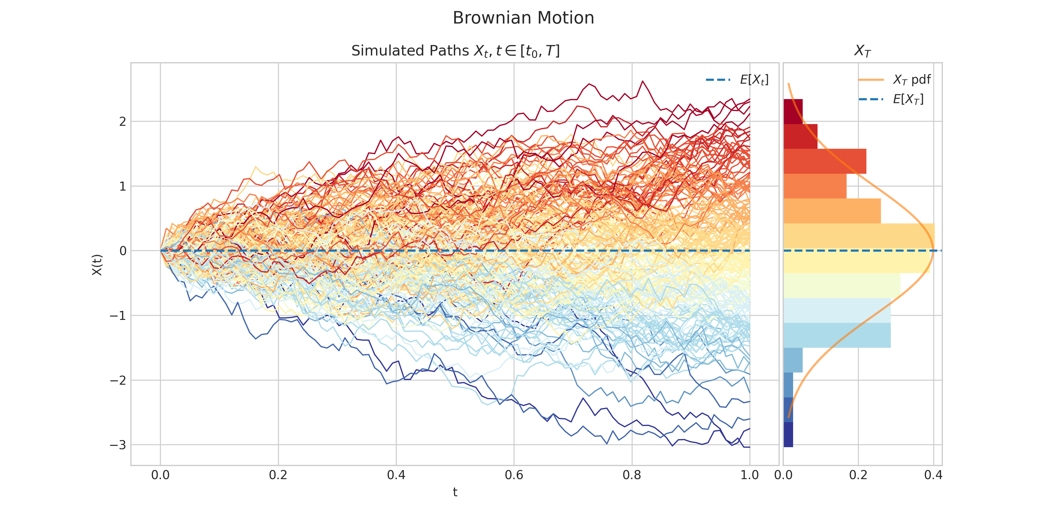
from aleatory.processes import BrownianMotion
process = BrownianMotion()
fig = process.draw(n=100, N=100, figsize=(12, 7))
fig.show()
Constructor, Methods, and Attributes#
- __init__(drift=0.0, scale=1.0, initial=0.0, T=1.0, rng=None)[source]#
- Parameters:
drift (double) – the drift parameter \(\mu\) in the above SDE
scale (double) – the scale parameter \(\sigma\) in the above SDE
initial (double) – the initial condition \(x_0\) in the above SDE
T (double) – the endpoint of the time interval \([0,T]\) over which the process is defined
rng – random number generator for reproducibility
Methods
__init__([drift, scale, initial, T, rng])- param double drift:
the drift parameter \(\mu\) in the above SDE
draw(n, N[, T, marginal, envelope, type, title])Simulates and plots paths/trajectories from the instanced stochastic process.
estimate_covariances([times])estimate_expectations()estimate_quantiles(q)estimate_stds()estimate_variances()get_marginal(t)marginal_expectation([times])marginal_stds([times])marginal_variance(times)plot(n, N[, T, title, suptitle])Simulates and plots paths/trajectories from the instanced stochastic process.
plot_covariance([times, title])plot_kernel([times, colormap, matrix_shape, ...])plot_kernel3d([times, title])plot_mean_variance(times, **fig_kw)plot_paths_and_kernel(n, N[, T, title, ...])Plots the paths of the process and the covariance kernel.
process_covariance([times])process_expectation()process_stds()process_variance()sample(n)Generates a discrete time sample from a Brownian Motion instance.
sample_at(times)Generates a sample from a Brownian motion at the specified times.
simulate(n, N[, T])Simulate paths/trajectories from the instanced stochastic process.
Attributes
TEnd time of the process.
driftinitialrngscale