Quick-Start Guide

To start using aleatory, import the stochastic processes you want and create an instance with the required parameters. For example, we create an instance of a standard Brownian motion as follows.

from aleatory.processes import BrownianMotion
brownian = BrownianMotion()

Note

All processes instances will be defined on a finite interval \([0,T]\). Hence, the end point \(T\) is a required argument to create an instance of a process. In all cases \(T=1,\) by default.

The simulate() method

Every process class has a simulate method to generate a number of trajectories/paths. The simulate methods require two parameters:

• n for the number of steps in each path

• N for the number of paths

and will return a list with N paths generated from the specified process.

For example, we can simulate 10 paths, each one with 100 steps, from a standard Brownian motion as follows.

from aleatory.processes import BrownianMotion

brownian = BrownianMotion()
paths = brownian.simulate(n=100, N=10)

Note

Each path is a numpy array which contains n points/steps corresponding to the values of the process at evenly spaced times over the interval \([0,T],\) i.e.,

\[\left\{X \left(\frac{i T }{n-1}\right), i=0,\cdots, n-1\right\}.\]

The plot() method

Every process class has a plot method for generating a simple chart with showing the required simulated trajectories/paths. Similarly to the simulate methods, the plot methods require two parameters:

• n for the number of steps in each path

• N for the number of paths

from aleatory.processes import BrownianMotion

brownian = BrownianMotion()
brownian.plot(n=100, N=10)

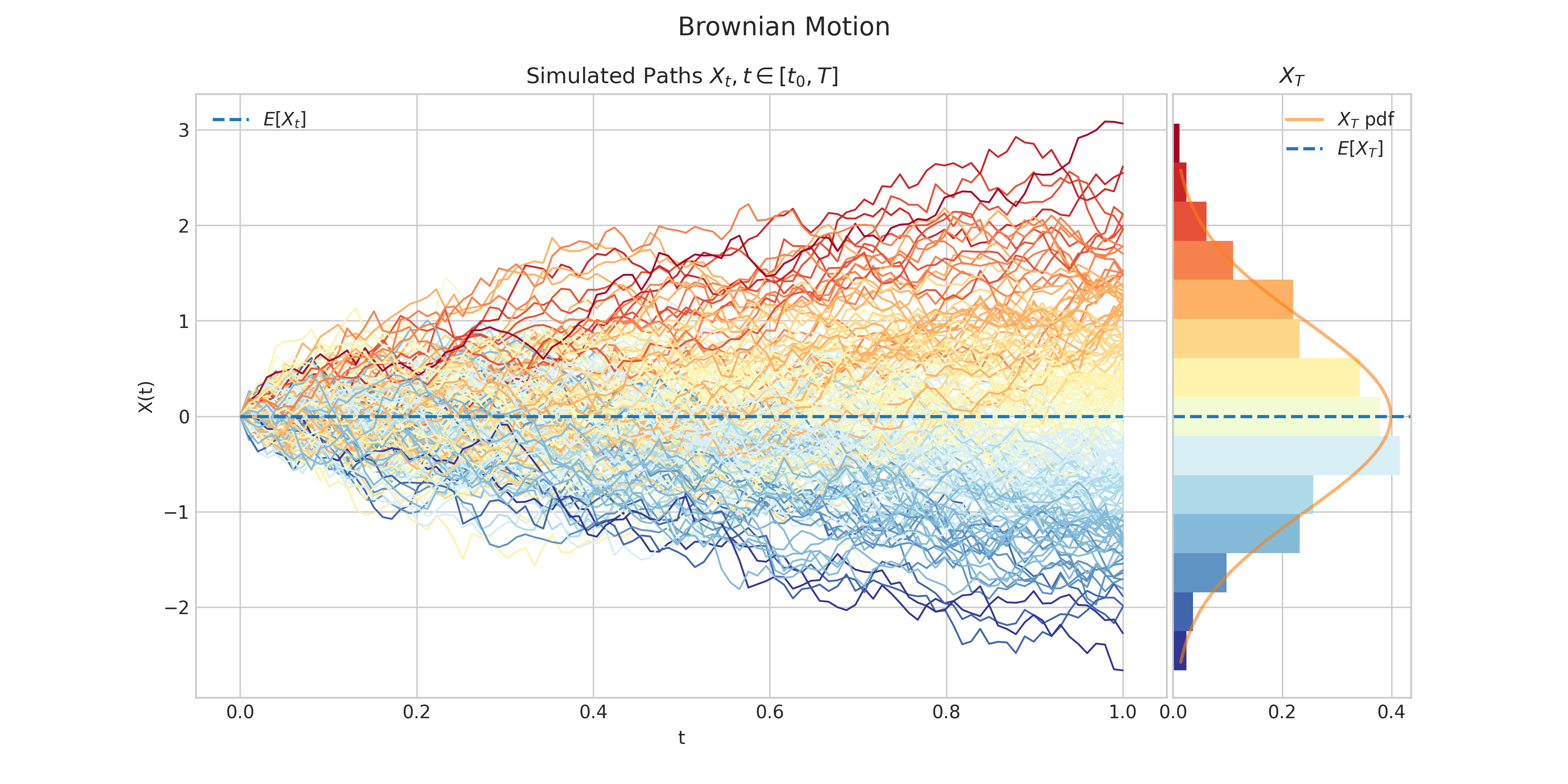
The draw() method

Every process class has a draw method which generates a more interesting visualisation of the simulated trajectories/paths.

The draw method also require two parameters:

• n for the number of steps in each path

• N for the number of paths

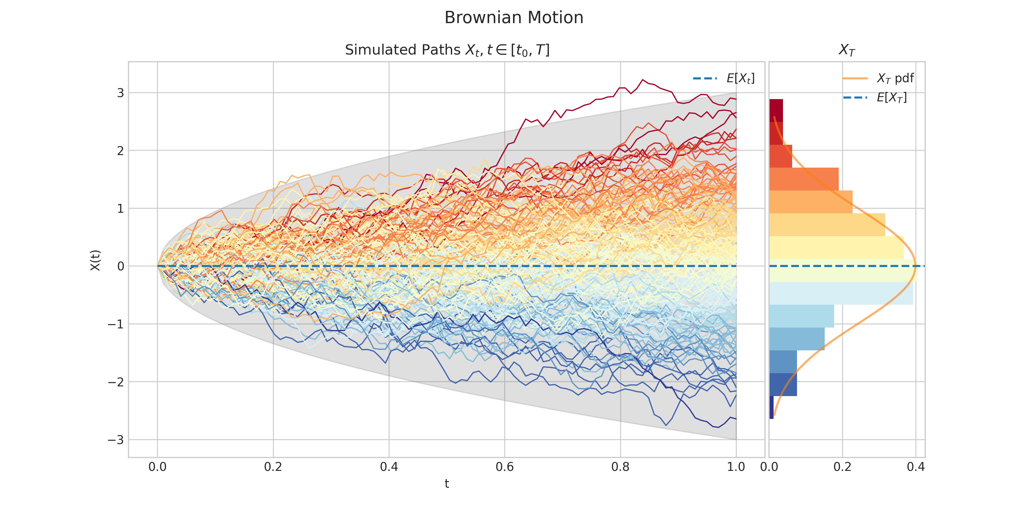
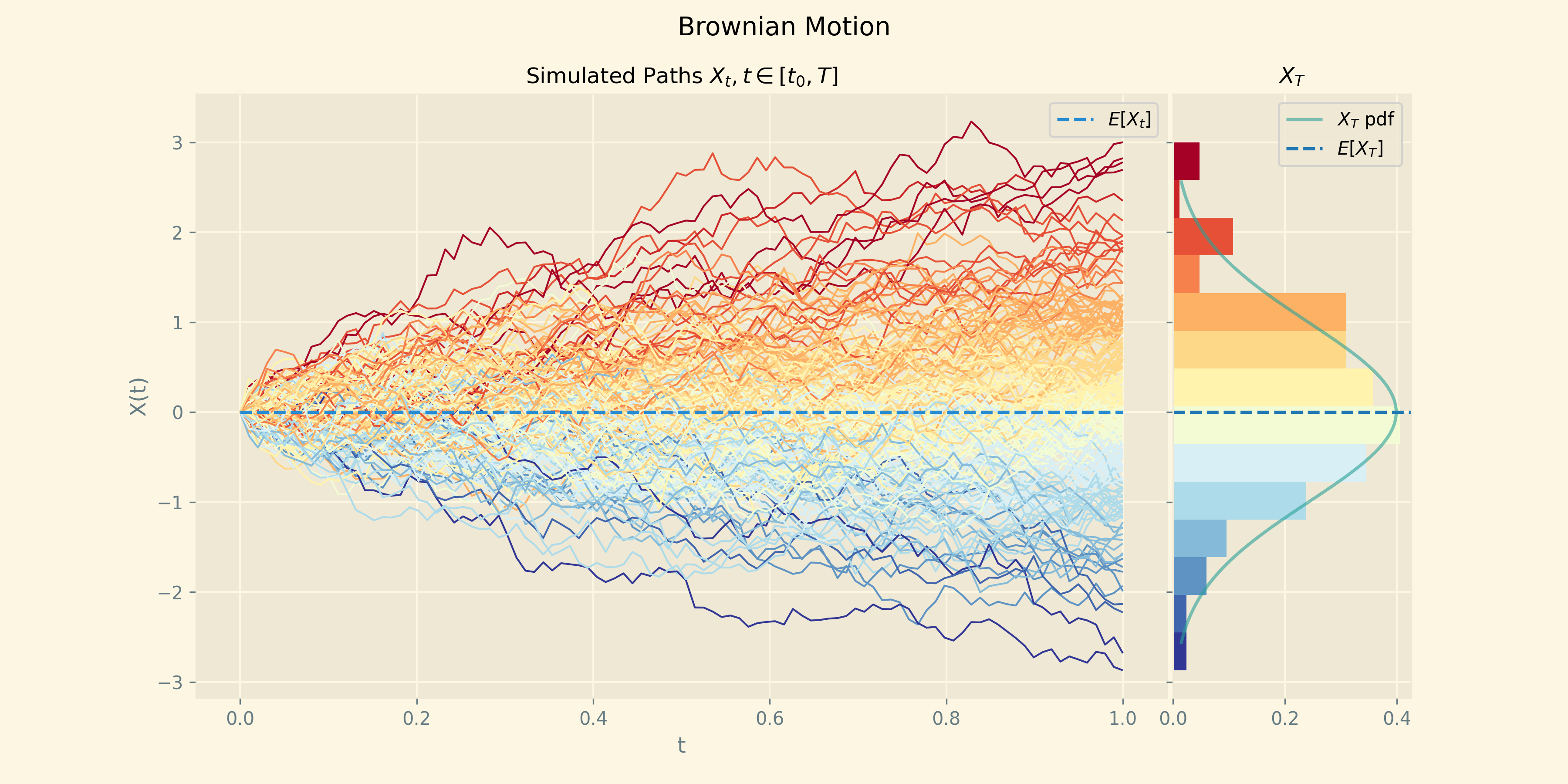
In addition, there are two optional boolean parameters

• marginal which enables/disables a subplot showing the marginal distribution of \(X_T\). This parameters is defaulted to True.

• envelope which enables/disables a the ability to show envelopes made of confidence intervals. This is defaulted to False`.

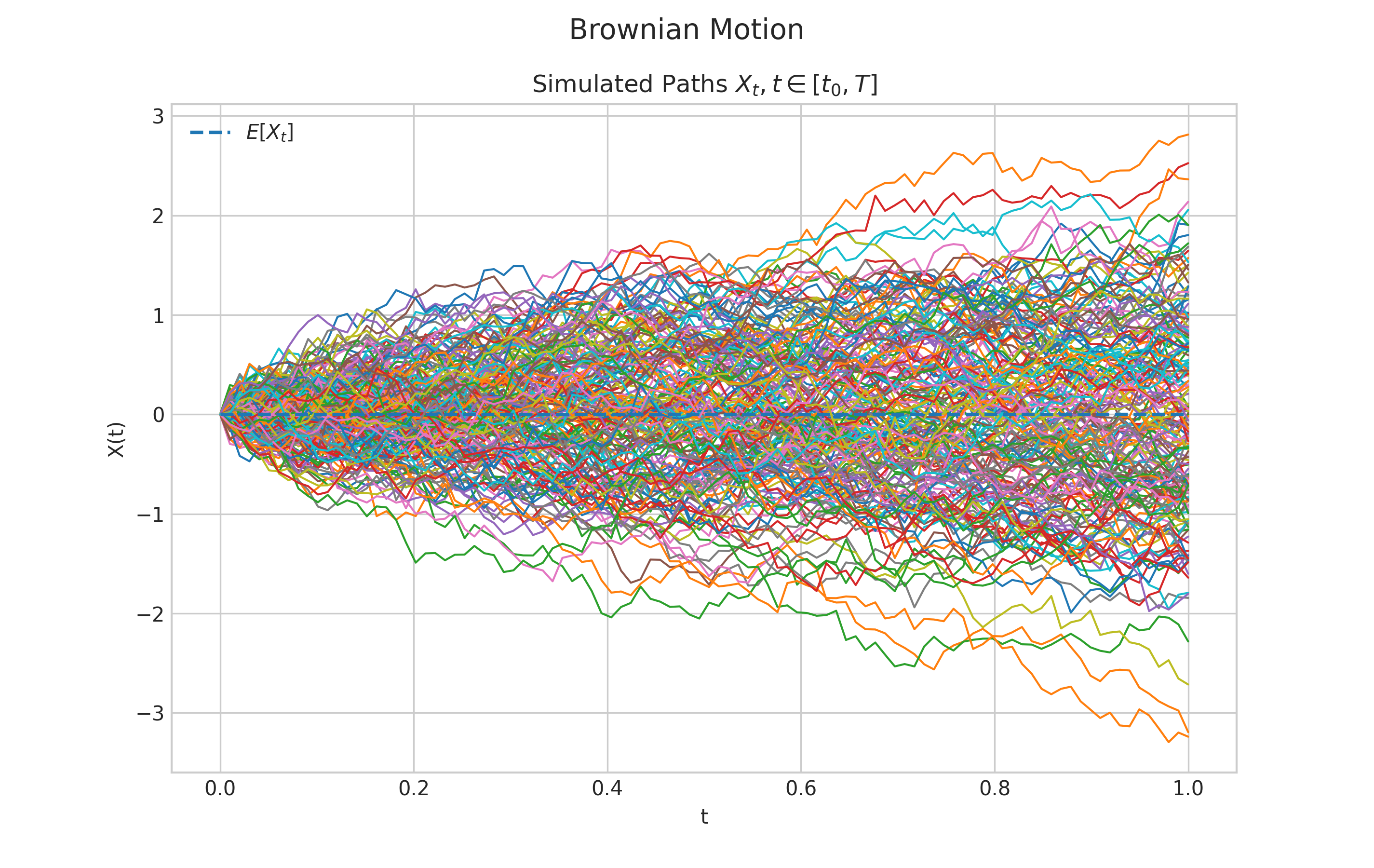
This allows us to produce four different charts.

from aleatory.processes import BrownianMotion

brownian = BrownianMotion()
brownian.draw(n=100, N=200)

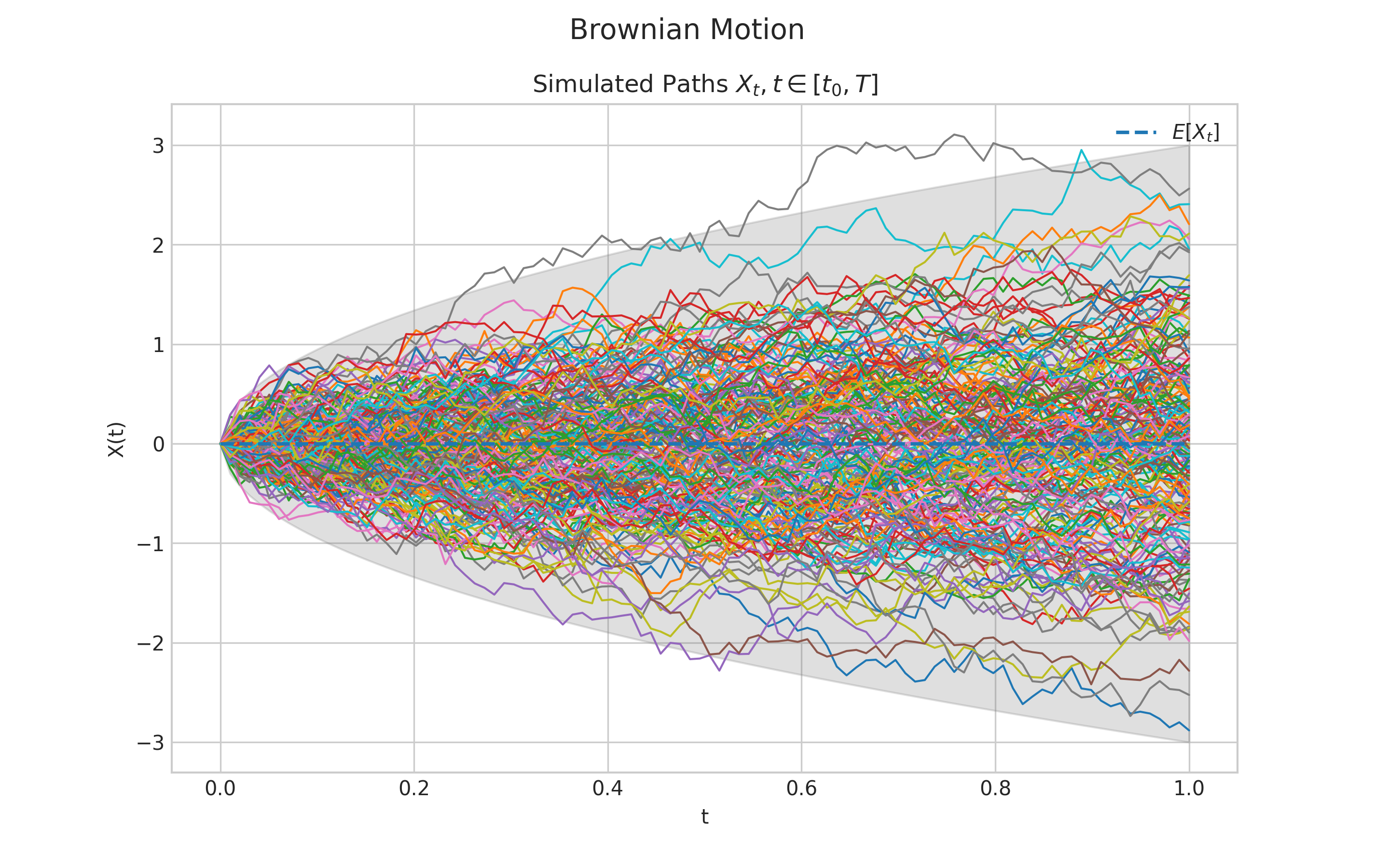
from aleatory.processes import BrownianMotion

brownian = BrownianMotion()
brownian.draw(n=100, N=200, envelope=True)

from aleatory.processes import BrownianMotion

brownian = BrownianMotion()
brownian.draw(n=100, N=200, marginal=False)

from aleatory.processes import BrownianMotion

brownian = BrownianMotion()
brownian.draw(n=100, N=200, marginal=False, envelope=True)

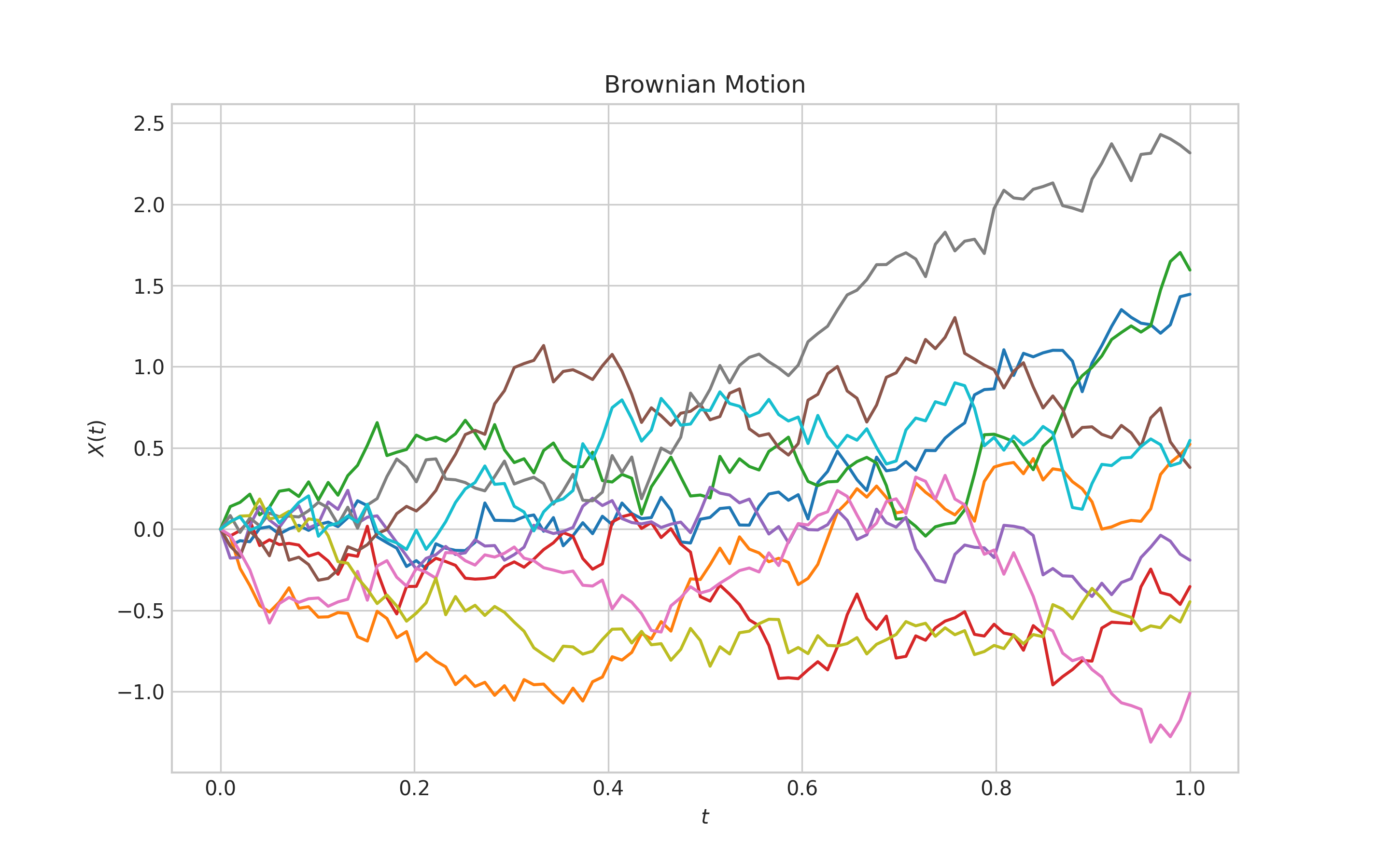
Charts Customisation

Both plot and draw methods allow chart customisation via a style parameter which leverages the style sheet feature.

The default style for all charts is "seaborn-v0_8-whitegrid". Visit the matplotlib Style sheet reference for more details and examples of the different styles.

from aleatory.processes import BrownianMotion

brownian = BrownianMotion()
brownian.plot(n=100, N=200, style='ggplot')

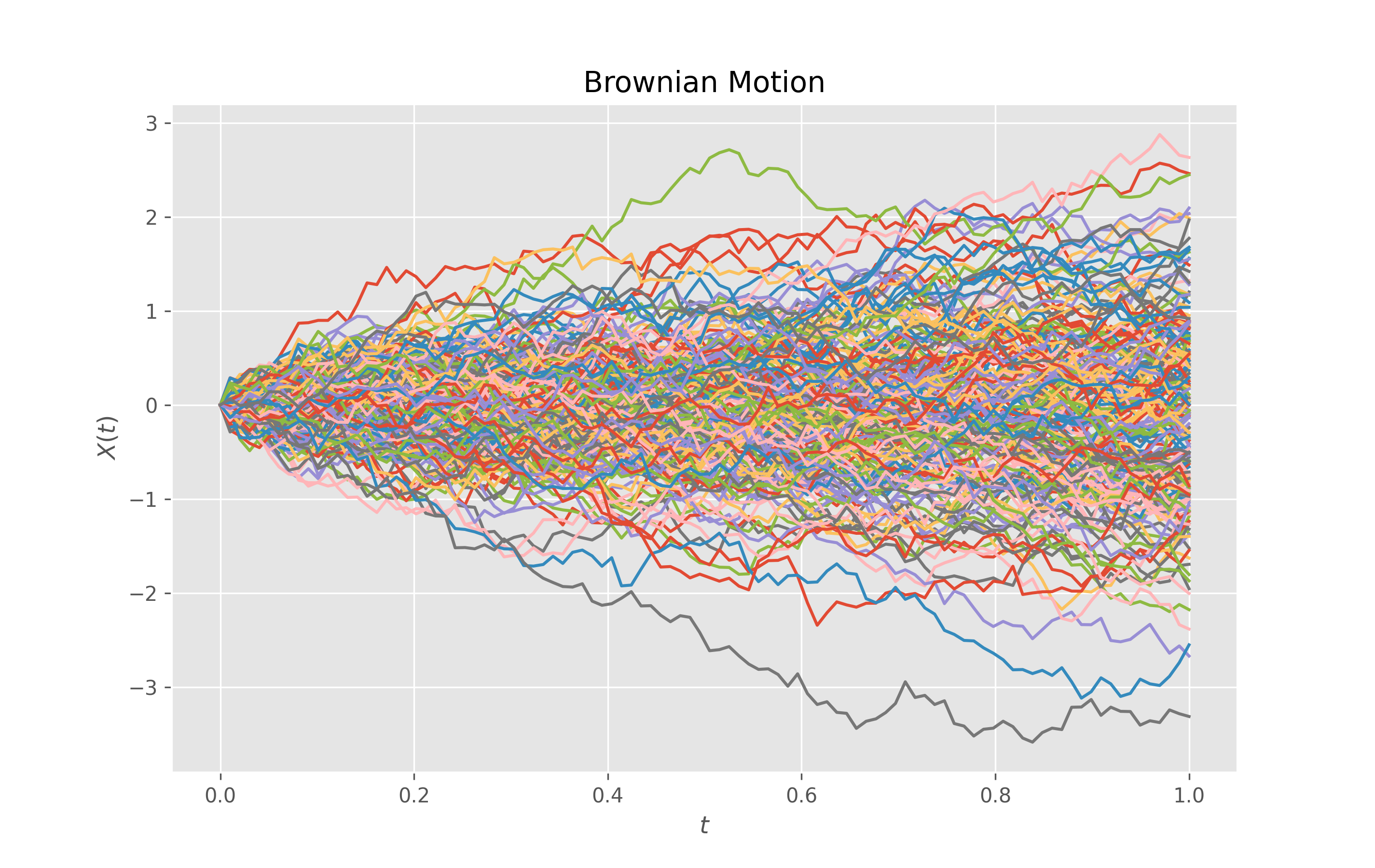
from aleatory.processes import BrownianMotion

brownian = BrownianMotion()
brownian.draw(n=100, N=100, style='Solarize_Light2')

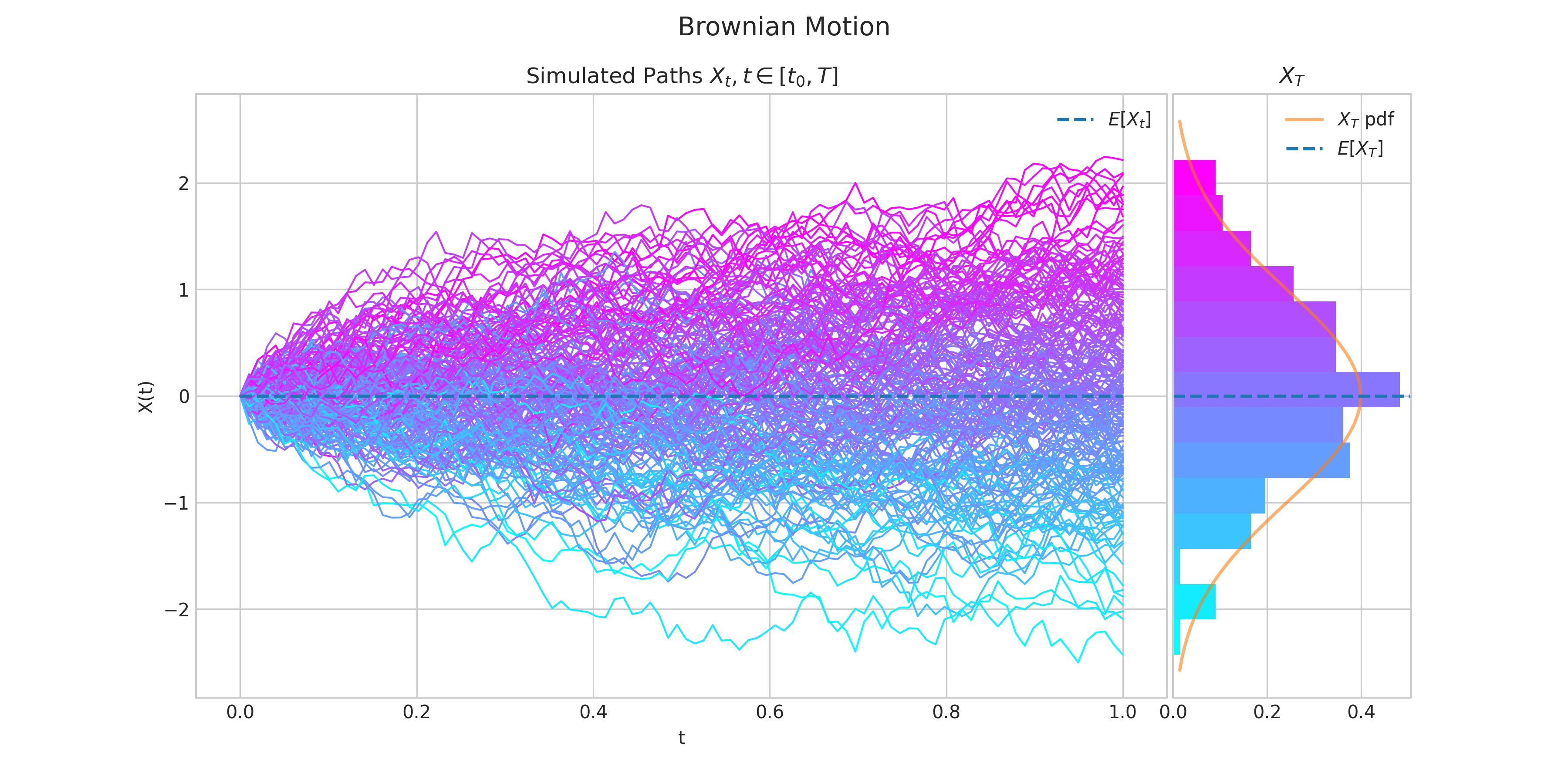
Finally, the method draw also offers the ability to customise the color map which is used. This is done via the parameter colormap

The default color map is "RdYlBu_r". Visit the matplotlib tutorial Choosing Colormaps in Matplotlib for more details and examples of the different color maps that you can use.

from aleatory.processes import BrownianMotion

brownian = BrownianMotion()
brownian.draw(n=100, N=100, colormap="cool")