CEV Process#

Simulate and visualise paths

# Author: Dialid Santiago <d.santiago@outlook.com>
# License: MIT
# Description: Simulate and visualise a CEV process

from aleatory.processes import CEVProcess
from aleatory.styles import qp_style

qp_style()  # Use quant-pastel-style

p = CEVProcess()
fig = p.draw(n=200, N=200, figsize=(12, 7), colormap="Purples")
fig.show()

$Constant Elasticity Variance (CEV) process $X(\mu=0.5, \gamma=1.5, \sigma=0.1)$ starting at 1.0, Monte Carlo Simulated Paths $\{{X_t, t \in [t_0, T]\}}$, $X_T$ Marginal$

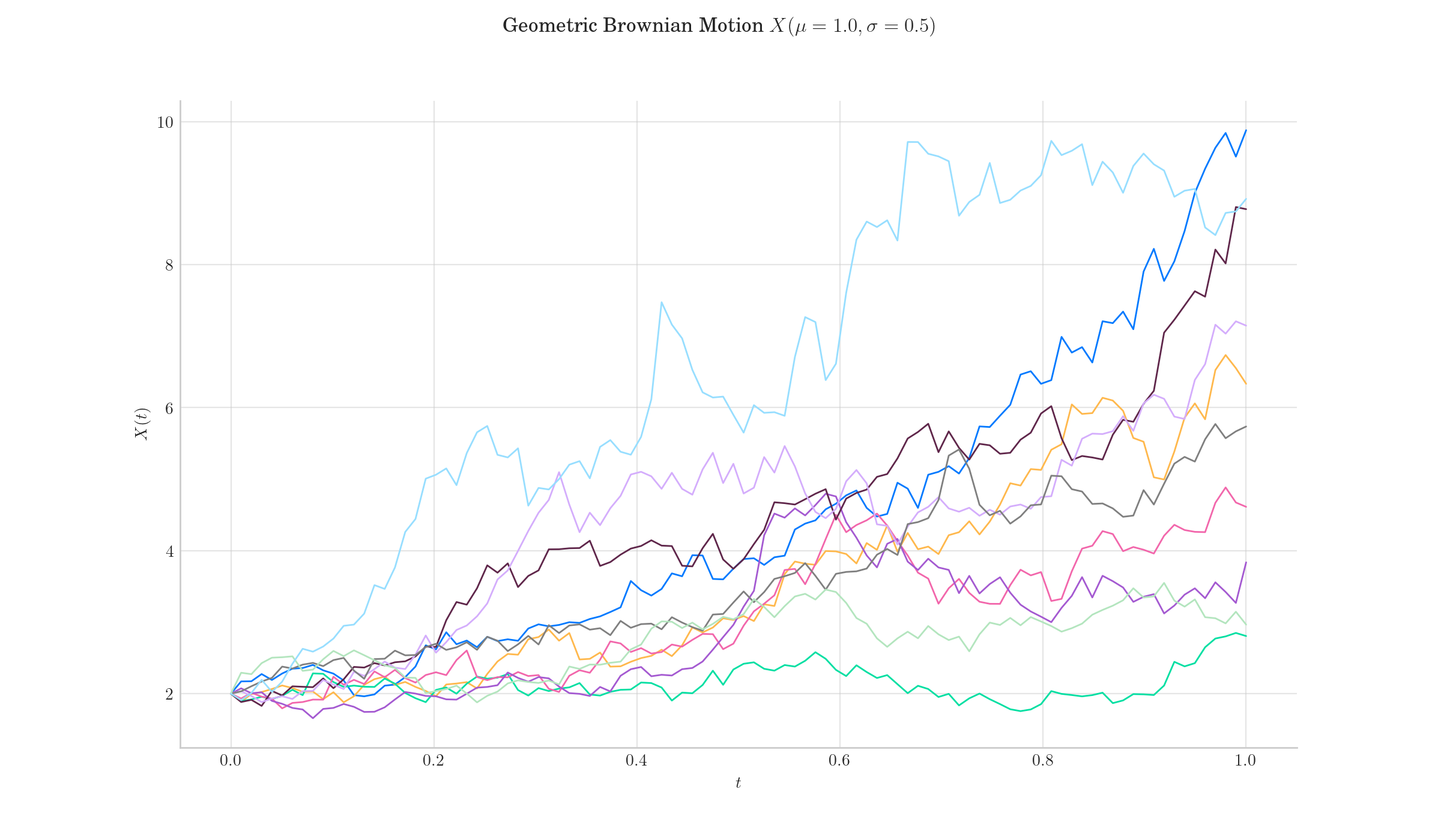
p = CEVProcess(mu=1.0, gamma=1.0, sigma=0.5, initial=2.0, T=1.0)
fig = p.draw(n=200, N=200, figsize=(12, 7), colormap="copper")
fig.show()

$Geometric Brownian Motion $X(\mu=1.0, \sigma=0.5)$, Monte Carlo Simulated Paths $\{{X_t, t \in [t_0, T]\}}$, $X_T$ Marginal$

fig = p.plot(n=100, N=10, figsize=(12, 7))
fig.show()

$Geometric Brownian Motion $X(\mu=1.0, \sigma=0.5)$$

Total running time of the script: (0 minutes 4.088 seconds)

Gallery generated by Sphinx-Gallery