Analytical Processes#
The aleatory.processes module provides classes for continuous-time stochastic processes which can be expressed in
analytical form.
- class aleatory.processes.BrownianMotion(drift=0.0, scale=1.0, T=1.0, rng=None)[source]#
Brownian motion
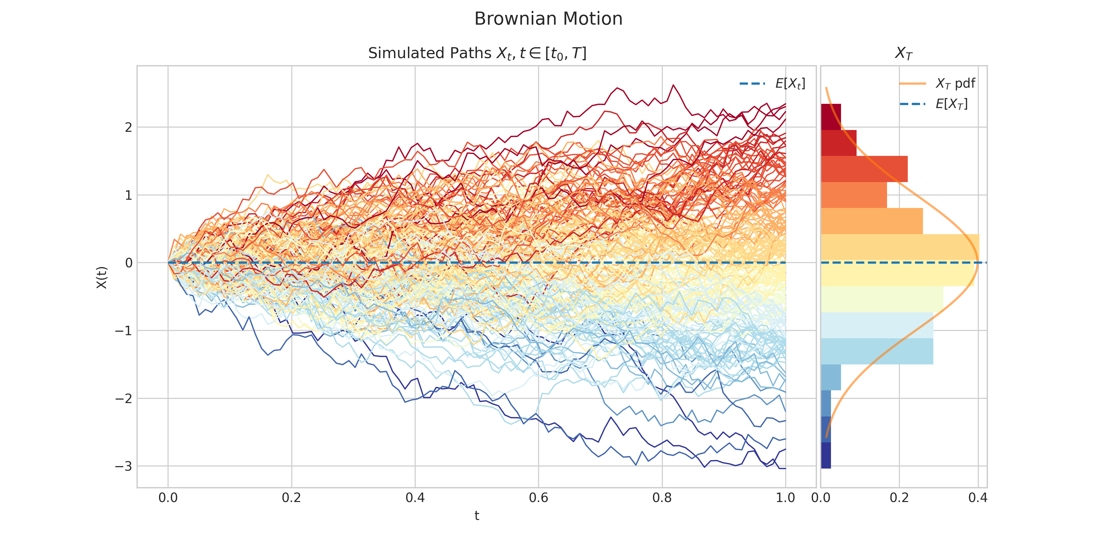
A standard Brownian motion \(\{W_t : t \geq 0\}\) is defined by the following properties:
Starts at zero, i.e. \(W(0) = 0\)
Independent increments
\(W(t) - W(s)\) follows a Gaussian distribution \(N(0, t-s)\)
Almost surely continuous
A more general version of a Brownian motion, is the Drifted Brownian Motion which is defined by the following SDE
\[dX_t = \mu dt + \sigma dW_t \ \ \ \ t\in (0,T]\]with initial condition \(X_0 = x_0\in\mathbb{R}\), where
\(\mu\) is the drift
\(\sigma>0\) is the volatility
\(W_t\) is a standard Brownian Motion.
Clearly, the solution to this equation can be written as
\[X_t = x_0 + \mu t + \sigma W_t \ \ \ \ t \in [0,T]\]and each \(X_t \sim N(\mu t, \sigma^2 t)\).
Parameters:
- Parameters:
drift (float) – the parameter \(\mu\) in the above SDE
scale (float) – the parameter \(\sigma>0\) in the above SDE
initial (float) – the initial condition \(x_0\) in the above SDE
T (float) – the right hand endpoint of the time interval \([0,T]\) for the process
rng (numpy.random.Generator) – a custom random number generator
- property T#
End time of the process.
- draw(n, N, marginal=True, envelope=False, type='3sigma', title=None, **fig_kw)[source]#
Simulates and plots paths/trajectories from the instanced stochastic process.
Produces different kind of visualisation illustrating the following elements:
times versus process values as lines
the expectation of the process across time
histogram showing the empirical marginal distribution \(X_T\) (optional when
marginal = True)probability density function of the marginal distribution \(X_T\) (optional when
marginal = True)envelope of confidence intervals across time (optional when
envelope = True)
- Parameters:
n – number of steps in each path
N – number of paths to simulate
marginal – bool, default: True
envelope – bool, default: False
type – string, default: ‘3sigma’
title – string to customise plot title
- Returns:
- plot(n, N, title=None, **fig_kw)#
Simulates and plots paths/trajectories from the instanced stochastic process. Simple plot of times versus process values as lines and/or markers.
- Parameters:
n – number of steps in each path
N – number of paths to simulate
title – string to customise plot title
- Returns:
- sample(n)[source]#
Generates a discrete time sample from a Brownian Motion instance.
- Parameters:
n – the number of steps
- Returns:
numpy array
- sample_at(times)[source]#
Generates a sample from a Brownian motion at the specified times.
- Parameters:
times – the times which define the sample
- Returns:
numpy array
- simulate(n, N)#
Simulate paths/trajectories from the instanced stochastic process.
- Parameters:
n – number of steps in each path
N – number of paths to simulate
- Returns:
list with N paths (each one is a numpy array of size n)
- class aleatory.processes.BrownianBridge(initial=0.0, end=0.0, T=1.0, rng=None)[source]#
Brownian Bridge
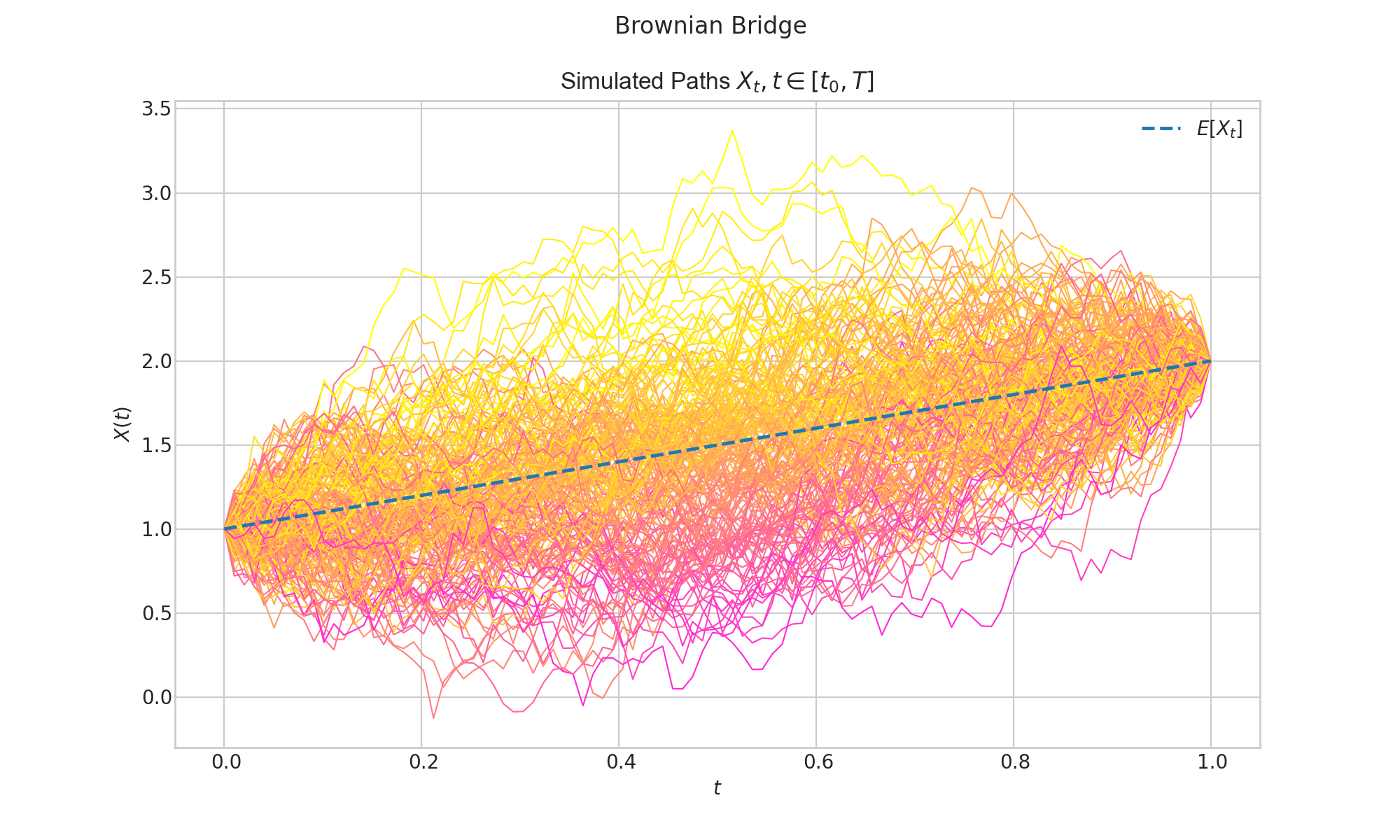
A Brownian bridge is a continuous-time stochastic process \(\{B_t : t \geq 0\}\) whose probability distribution is the conditional probability distribution of a standard Wiener process (Brownian Motion) \(\{W_t : t \geq 0\}\) subject to the condition that \(W(T) = 0\), so that the process is pinned to the same value at both \(t = 0\) and \(t = T\). More specifically,
\[B_t = (W_t | W_T = 0), \ \ \ \ t\in (0,T].\]More generally, a Brownian Bridge is subject to the conditions \(W(0) = a\) and \(W(T) = b\).
- Parameters
- param float initial:
initial condition
- param float end:
end condition
- param float T:
the right hand endpoint of the time interval \([0,T]\)
for the process :param numpy.random.Generator rng: a custom random number generator
- property T#
End time of the process.
- draw(n, N, envelope=False, title=None, **fig_kw)[source]#
Simulates and plots paths/trajectories from the instanced stochastic process.
Produces different kind of visualisation illustrating the following elements:
times versus process values as lines
the expectation of the process across time
envelope of confidence intervals across time (optional when
envelope = True)
- Parameters:
n – number of steps in each path
N – number of paths to simulate
envelope – bool, default: False
title – string to customise plot title
- Returns:
- plot(n, N, title=None, **fig_kw)#
Simulates and plots paths/trajectories from the instanced stochastic process. Simple plot of times versus process values as lines and/or markers.
- Parameters:
n – number of steps in each path
N – number of paths to simulate
title – string to customise plot title
- Returns:
- sample(n)[source]#
Generates a discrete time sample from a Brownian Motion instance.
- Parameters:
n – the number of steps
- Returns:
numpy array
- sample_at(times)[source]#
Generates a sample from a Brownian motion at the specified times.
- Parameters:
times – the times which define the sample
- Returns:
numpy array
- simulate(n, N)#
Simulate paths/trajectories from the instanced stochastic process.
- Parameters:
n – number of steps in each path
N – number of paths to simulate
- Returns:
list with N paths (each one is a numpy array of size n)
- class aleatory.processes.BrownianExcursion(T=1.0, rng=None)[source]#
Brownian Excursion
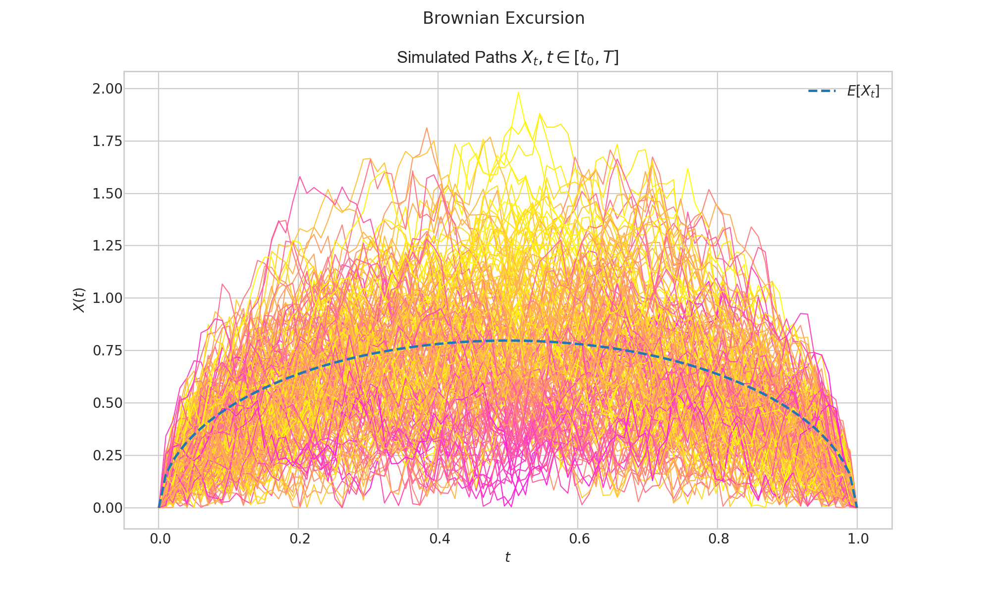
A Brownian excursion process, is a Wiener process (or Brownian motion) conditioned to be positive and to take the value 0 at time 1. Alternatively, it can be defined as a Brownian Bridge process conditioned to be positive.
- Parameters
- param float T:
the right hand endpoint of the time interval \([0,T]\)
for the process :param numpy.random.Generator rng: a custom random number generator
- property T#
End time of the process.
- draw(n, N, envelope=False, title=None, **fig_kw)#
Simulates and plots paths/trajectories from the instanced stochastic process.
Produces different kind of visualisation illustrating the following elements:
times versus process values as lines
the expectation of the process across time
envelope of confidence intervals across time (optional when
envelope = True)
- Parameters:
n – number of steps in each path
N – number of paths to simulate
envelope – bool, default: False
title – string to customise plot title
- Returns:
- plot(n, N, title=None, **fig_kw)#
Simulates and plots paths/trajectories from the instanced stochastic process. Simple plot of times versus process values as lines and/or markers.
- Parameters:
n – number of steps in each path
N – number of paths to simulate
title – string to customise plot title
- Returns:
- sample(n)[source]#
Generates a discrete time sample from a Brownian Motion instance.
- Parameters:
n – the number of steps
- Returns:
numpy array
- sample_at(times)[source]#
Generates a sample from a Brownian motion at the specified times.
- Parameters:
times – the times which define the sample
- Returns:
numpy array
- simulate(n, N)#
Simulate paths/trajectories from the instanced stochastic process.
- Parameters:
n – number of steps in each path
N – number of paths to simulate
- Returns:
list with N paths (each one is a numpy array of size n)
- class aleatory.processes.BrownianMeander(T=1.0, fixed_end=False, end=None, rng=None)[source]#
Brownian Meander
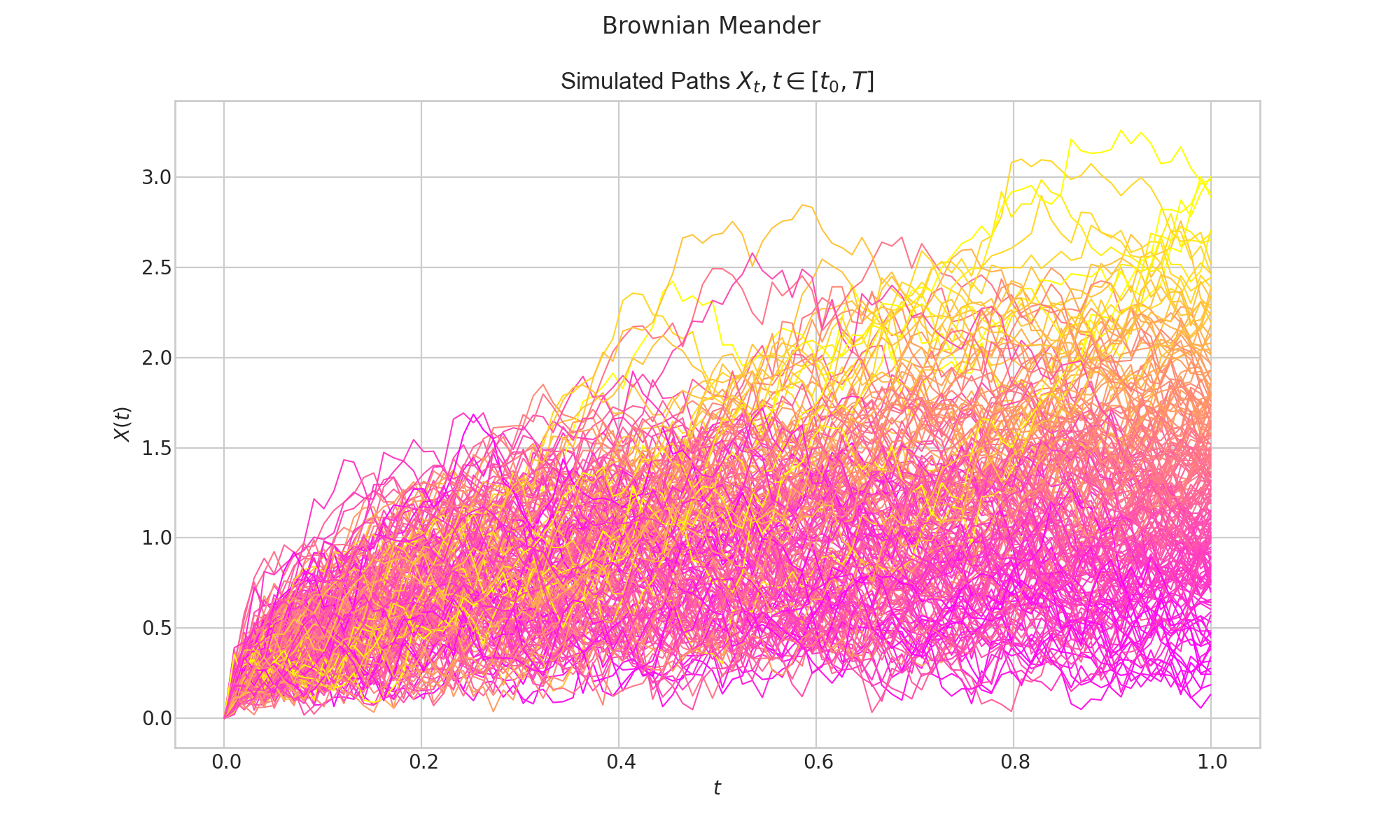
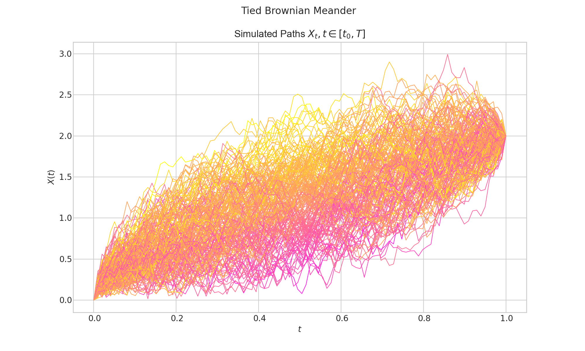
Let \(\{W_t : t \geq 0\}\) be a standard Brownian motion and
\[\tau = \sup\{ t \in [0,1] : W_t =0\},\]i.e. the last time before t = 1 when \(W_t\) visits zero. Then the Brownian Meander is defined as follows
\[W_t^{+} = \frac{1}{\sqrt{1-\tau}} |W(\tau + t (1-\tau))|, \ \ \ \ t\in (0,1].\]Parameters
- property T#
End time of the process.
- draw(n, N, title=None, **fig_kw)[source]#
Simulates and plots paths/trajectories from the instanced stochastic process.
Produces different kind of visualisation illustrating the following elements:
times versus process values as lines
the expectation of the process across time
histogram showing the empirical marginal distribution \(X_T\) (optional when
marginal = True)probability density function of the marginal distribution \(X_T\) (optional when
marginal = True)envelope of confidence intervals across time (optional when
envelope = True)
- Parameters:
n – number of steps in each path
N – number of paths to simulate
title – string to customise plot title
- Returns:
- plot(n, N, title=None, **fig_kw)#
Simulates and plots paths/trajectories from the instanced stochastic process. Simple plot of times versus process values as lines and/or markers.
- Parameters:
n – number of steps in each path
N – number of paths to simulate
title – string to customise plot title
- Returns:
- sample(n)[source]#
Generates a discrete time sample from a Brownian Motion instance.
- Parameters:
n – the number of steps
- Returns:
numpy array
- sample_at(times)[source]#
Generates a sample from a Brownian motion at the specified times.
- Parameters:
times – the times which define the sample
- Returns:
numpy array
- simulate(n, N)#
Simulate paths/trajectories from the instanced stochastic process.
- Parameters:
n – number of steps in each path
N – number of paths to simulate
- Returns:
list with N paths (each one is a numpy array of size n)
- class aleatory.processes.GBM(drift=1.0, volatility=0.5, initial=1.0, T=1.0, rng=None)[source]#
Geometric Brownian Motion
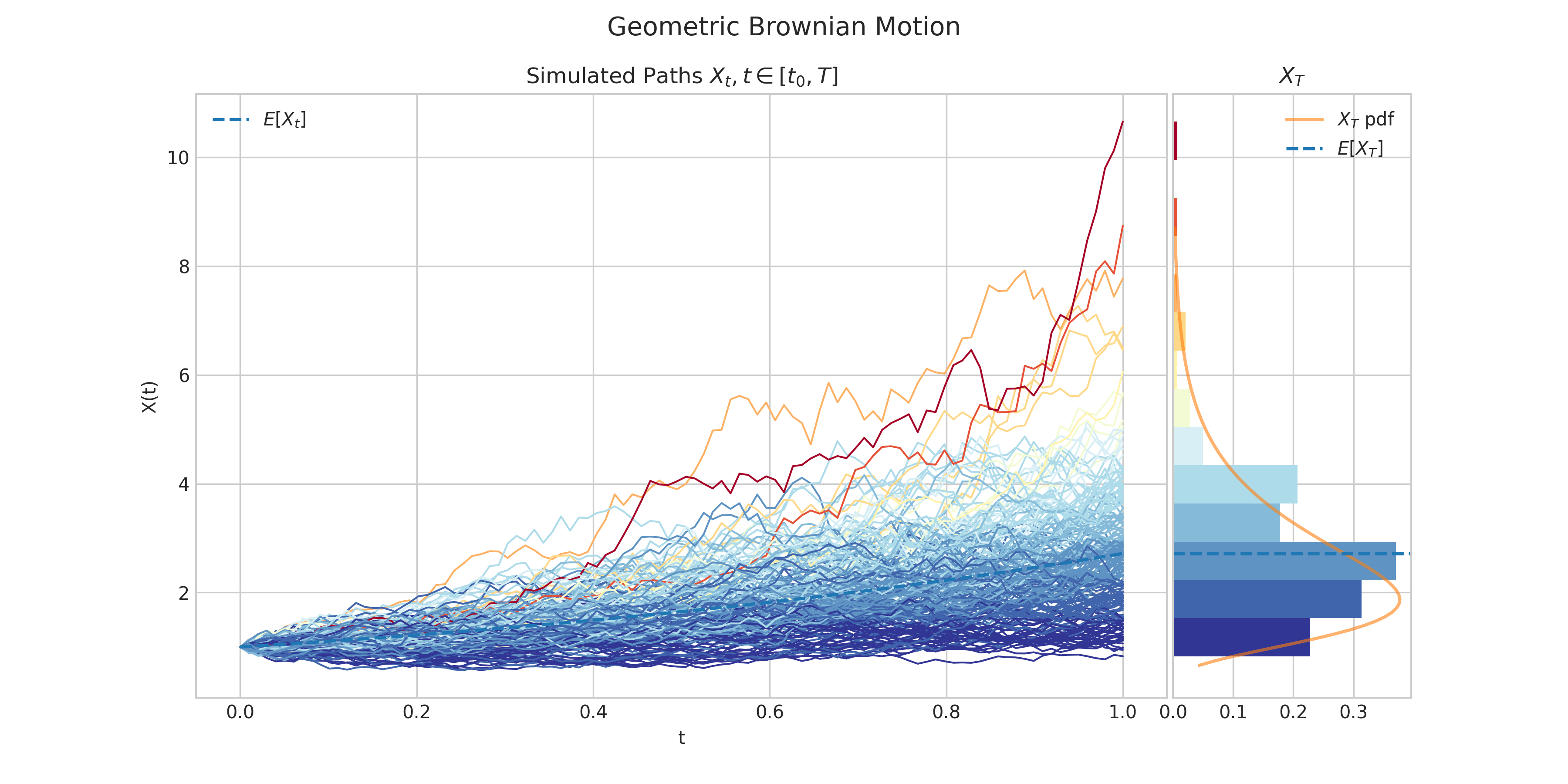
A Geometric Brownian Motion \(\{X(t) : t \geq 0\}\) is characterised by the following SDE.
\[dX_t = \mu X_t dt + \sigma X_t dW_t \ \ \ \ t\in (0,T]\]with initial condition \(X_0 = x_0\geq0\), where
\(\mu\) is the drift
\(\sigma>0\) is the volatility
\(W_t\) is a standard Brownian Motion.
The solution to this equation can be written as
\[X_t = x_0\exp\left((\mu + \frac{\sigma^2}{2} )t +\sigma W_t\right)\]and each \(X_t\) follows a log-normal distribution.
- Parameters:
drift (float) – the parameter \(\mu\) in the above SDE
volatility (float) – the parameter \(\sigma>0\) in the above SDE
initial (float) – the initial condition \(x_0\) in the above SDE
T (float) – the right hand endpoint of the time interval \([0,T]\) for the process
rng (numpy.random.Generator) – a custom random number generator
- property T#
End time of the process.
- draw(n, N, marginal=True, envelope=False, title=None, **fig_kw)#
Simulates and plots paths/trajectories from the instanced stochastic process. Visualisation shows - times versus process values as lines - the expectation of the process across time - histogram showing the empirical marginal distribution \(X_T\) - probability density function of the marginal distribution \(X_T\) - envelope of confidence intervals
- Parameters:
n – number of steps in each path
N – number of paths to simulate
marginal – bool, default: True
envelope – bool, default: False
title – string optional default to None
- Returns:
- plot(n, N, title=None, **fig_kw)#
Simulates and plots paths/trajectories from the instanced stochastic process. Simple plot of times versus process values as lines and/or markers.
- Parameters:
n – number of steps in each path
N – number of paths to simulate
title – string to customise plot title
- Returns:
- simulate(n, N)#
Simulate paths/trajectories from the instanced stochastic process.
- Parameters:
n – number of steps in each path
N – number of paths to simulate
- Returns:
list with N paths (each one is a numpy array of size n)
- class aleatory.processes.BESProcess(dim=1.0, initial=0.0, T=1.0, rng=None)[source]#
Bessel process
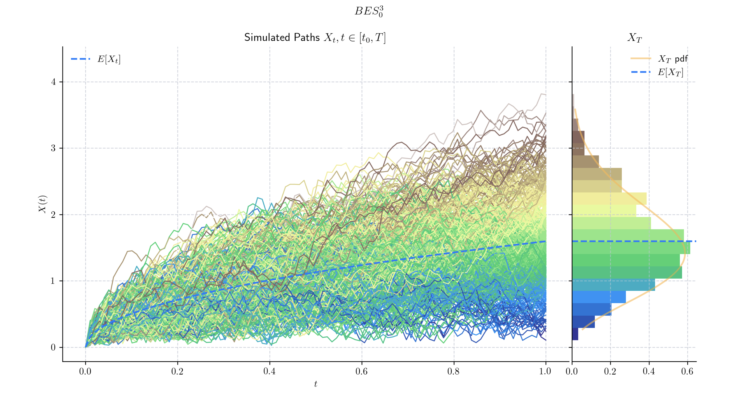
A Bessel process \(BES^{n}_{0},\) for \(n\geq 2\) integer is a continuous stochastic process \(\{X(t) : t \geq 0\}\) characterised as the Euclidian norm of an \(n\)-dimensional Brownian motion. That is,
\[X_t = \sqrt{\sum_{i=1}^n (W^i_t)^2}.\]More generally, for any \(\delta >0\), and \(x_0 \geq 0\), a Bessel process of dimension \(\delta\) starting at \(x_0\), denoted by
\[BES_{{x_0}}^{{\delta}}\]can be defined by the following SDE
\[dX_t = \frac{(\delta-1)}{2} \frac{dt}{X_t} + dW_t \ \ \ \ t\in (0,T]\]with initial condition \(X_0 = x_0\geq 0.\), where
\(\delta\) is a positive real
\(W_t\) is a standard one-dimensional Brownian Motion.
- Parameters:
dim (double) – the dimension of the process \(n\)
initial (double) – the initial point of the process \(x_0\)
T (double) – the right hand endpoint of the time interval \([0,T]\) for the process
rng (numpy.random.Generator) – a custom random number generator
- property T#
End time of the process.
- draw(n, N, marginal=True, envelope=False, title=None, **fig_kw)#
Simulates and plots paths/trajectories from the instanced stochastic process. Visualisation shows - times versus process values as lines - the expectation of the process across time - histogram showing the empirical marginal distribution \(X_T\) - probability density function of the marginal distribution \(X_T\) - envelope of confidence intervals
- Parameters:
n – number of steps in each path
N – number of paths to simulate
marginal – bool, default: True
envelope – bool, default: False
title – string optional default to None
- Returns:
- plot(n, N, title=None, **fig_kw)#
Simulates and plots paths/trajectories from the instanced stochastic process. Simple plot of times versus process values as lines and/or markers.
- Parameters:
n – number of steps in each path
N – number of paths to simulate
title – string to customise plot title
- Returns:
- class aleatory.processes.BESQProcess(dim=1.0, initial=0.0, T=1.0, rng=None)[source]#
Squared Bessel process
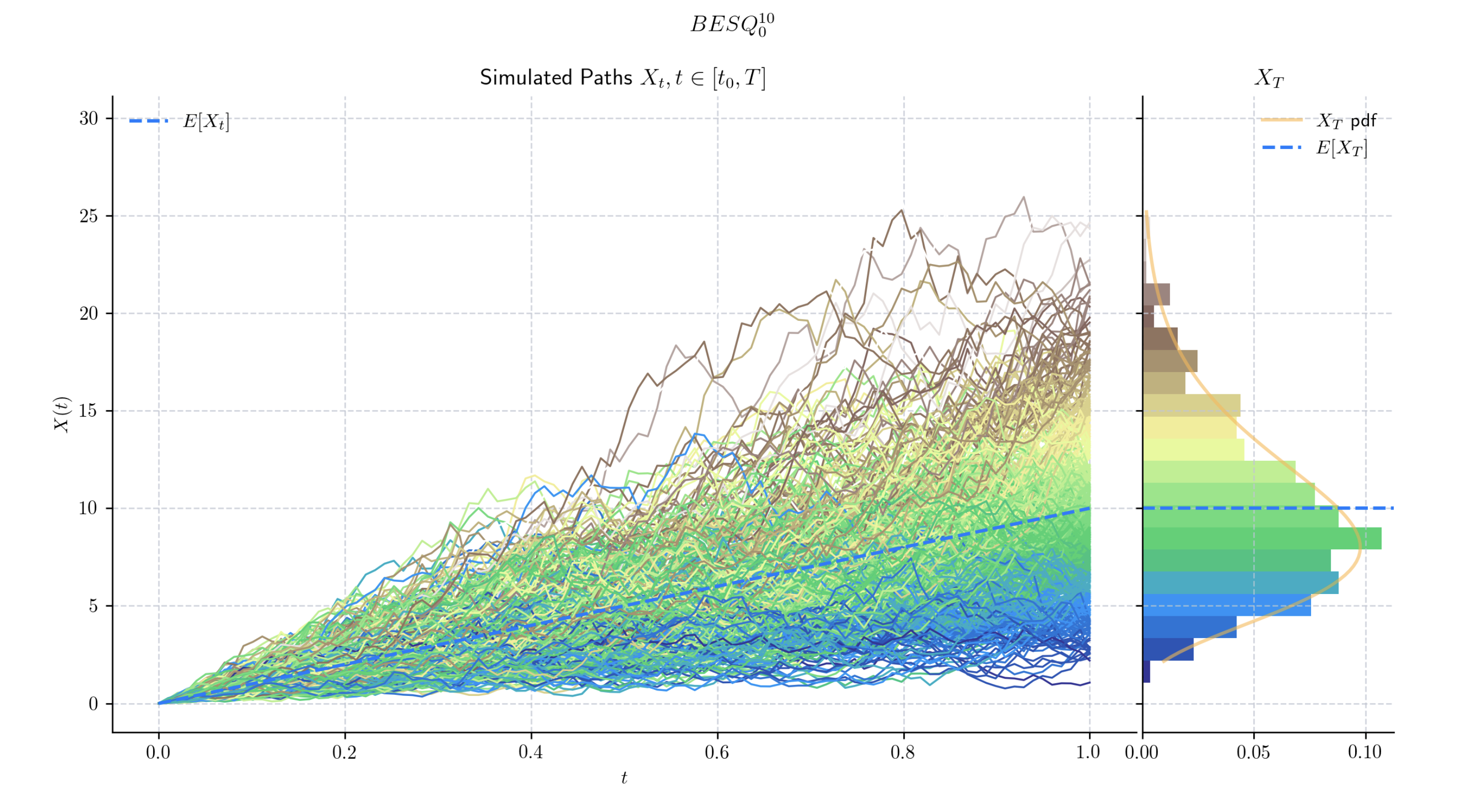
A squared Bessel process \(BESQ^{n}_{0}\), for \(n\) integer is a continuous stochastic process \(\{X(t) : t \geq 0\}\) which is characterised as the squared Euclidian norm of an \(n\)-dimensional Brownian motion. That is,
\[X_t = \sum_{i=1}^n (W^i_t)^2.\]More generally, for any \(\delta >0\), and \(x_0 \geq 0\), a squared Bessel process of dimension \(\delta\) starting at \(x_0\), denoted by
\[BESQ_{{x_0}}^{{\delta}}\]can be defined by the following SDE
\[dX_t = \delta dt + 2\sqrt{X_t} dW_t \ \ \ \ t\in (0,T]\]with initial condition \(X_0 = x_0\), where
\(\delta\) is a positive real
\(W_t\) is a standard Brownian Motion.
- Parameters:
dim (double) – the dimension of the process \(n\)
initial (double) – the initial point of the process \(x_0\)
T (double) – the right hand endpoint of the time interval \([0,T]\) for the process
rng (numpy.random.Generator) – a custom random number generator
- property T#
End time of the process.
- draw(n, N, marginal=True, envelope=False, title=None, **fig_kw)#
Simulates and plots paths/trajectories from the instanced stochastic process. Visualisation shows - times versus process values as lines - the expectation of the process across time - histogram showing the empirical marginal distribution \(X_T\) - probability density function of the marginal distribution \(X_T\) - envelope of confidence intervals
- Parameters:
n – number of steps in each path
N – number of paths to simulate
marginal – bool, default: True
envelope – bool, default: False
title – string optional default to None
- Returns:
- plot(n, N, title=None, **fig_kw)#
Simulates and plots paths/trajectories from the instanced stochastic process. Simple plot of times versus process values as lines and/or markers.
- Parameters:
n – number of steps in each path
N – number of paths to simulate
title – string to customise plot title
- Returns: