EM Processes#
The aleatory.processes module also provides functionality for continuous-time stochastic processes which
cannot be expressed in analytical form. These processes are simulated via the
Euler-Maruyama method.
- class aleatory.processes.OUProcess(theta=1.0, sigma=0.5, initial=1.0, T=1.0, rng=None)[source]#
Ornstein–Uhlenbeck Process
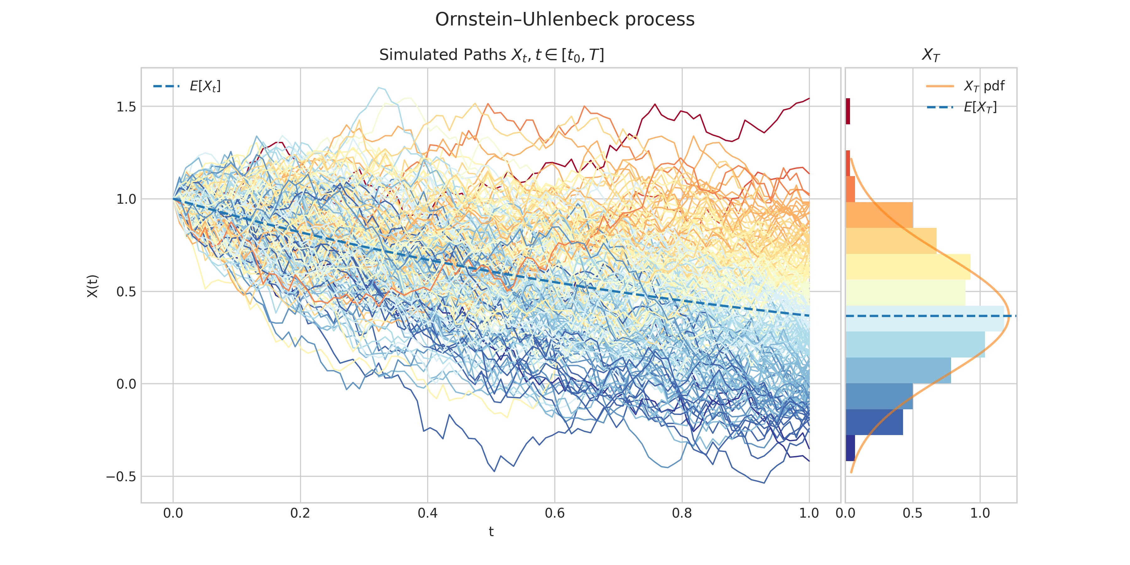
An Ornstein–Uhlenbeck process \(X = \{X : t \geq 0\}\) is characterised by the following Stochastic Differential Equation
\[dX_t = -\theta X_t dt + \sigma X_t dW_t, \ \ \ \ \forall t\in (0,T],\]with initial condition \(X_0 = x_0\), where
\(\theta\) is the speed of reversion
\(\sigma>0\) is the instantaneous volatility
\(W_t\) is a standard Brownian Motion.
Each \(X_t\) follows a normal distribution.
- Parameters:
theta (float) – the parameter \(\theta\) in the above SDE
sigma (float) – the parameter \(\sigma>0\) in the above SDE
initial (float) – the initial condition \(x_0\) in the above SDE
T (float) – the right hand endpoint of the time interval \([0,T]\) for the process
rng (numpy.random.Generator) – a custom random number generator
- property T#
End time of the process.
- draw(n, N, marginal=True, envelope=False, title=None, **fig_kw)#
Simulates and plots paths/trajectories from the instanced stochastic process. Visualisation shows - times versus process values as lines - the expectation of the process across time - histogram showing the empirical marginal distribution \(X_T\) - probability density function of the marginal distribution \(X_T\) - envelope of confidence intervals
- Parameters:
n – number of steps in each path
N – number of paths to simulate
marginal – bool, default: True
envelope – bool, default: False
title – string optional default to None
- Returns:
- plot(n, N, title=None, **fig_kw)#
Simulates and plots paths/trajectories from the instanced stochastic process. Simple plot of times versus process values as lines and/or markers.
- Parameters:
n – number of steps in each path
N – number of paths to simulate
title – string to customise plot title
- Returns:
- simulate(n, N)#
Simulate paths/trajectories from the instanced stochastic process.
- Parameters:
n – number of steps in each path
N – number of paths to simulate
- Returns:
list with N paths (each one is a numpy array of size n)
- class aleatory.processes.Vasicek(theta=1.0, mu=3.0, sigma=0.5, initial=1.0, T=1.0, rng=None)[source]#
Vasicek Process
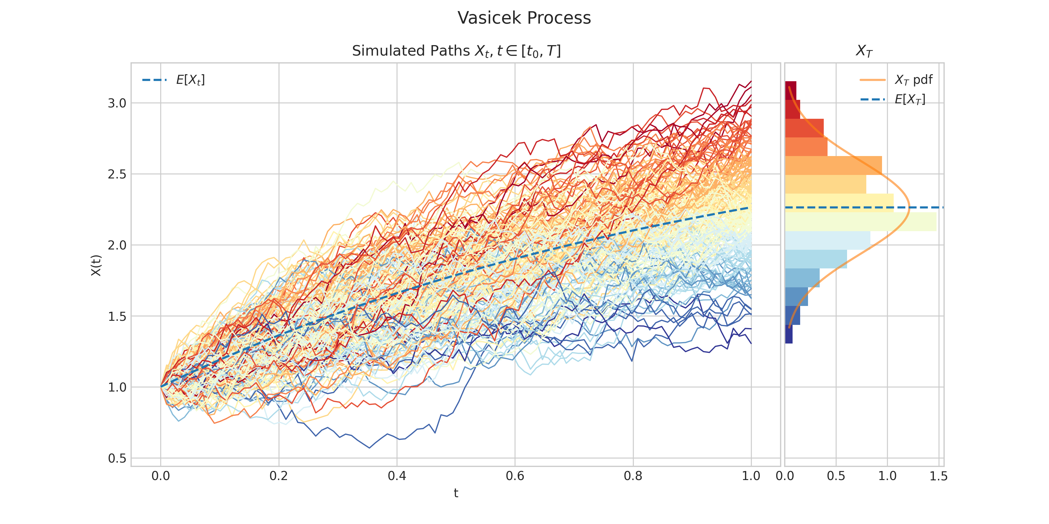
A Vasicek process \(X = \{X : t \geq 0\}\) is characterised by the following Stochastic Differential Equation
\[dX_t = \theta(\mu - X_t) dt + \sigma dW_t, \ \ \ \ \forall t\in (0,T],\]with initial condition \(X_0 = x_0\), where
\(\theta\) is the speed of reversion
\(\mu\) is the long term mean value.
\(\sigma>0\) is the instantaneous volatility
\(W_t\) is a standard Brownian Motion.
Each \(X_t\) follows a normal distribution.
- Parameters:
theta (float) – the parameter \(\theta\) in the above SDE
mu (float) – the parameter \(\mu\) in the above SDE
sigma (float) – the parameter \(\sigma>0\) in the above SDE
initial (float) – the initial condition \(x_0\) in the above SDE
T (float) – the right hand endpoint of the time interval \([0,T]\) for the process
rng (numpy.random.Generator) – a custom random number generator
- property T#
End time of the process.
- draw(n, N, marginal=True, envelope=False, title=None, **fig_kw)#
Simulates and plots paths/trajectories from the instanced stochastic process. Visualisation shows - times versus process values as lines - the expectation of the process across time - histogram showing the empirical marginal distribution \(X_T\) - probability density function of the marginal distribution \(X_T\) - envelope of confidence intervals
- Parameters:
n – number of steps in each path
N – number of paths to simulate
marginal – bool, default: True
envelope – bool, default: False
title – string optional default to None
- Returns:
- plot(n, N, title=None, **fig_kw)#
Simulates and plots paths/trajectories from the instanced stochastic process. Simple plot of times versus process values as lines and/or markers.
- Parameters:
n – number of steps in each path
N – number of paths to simulate
title – string to customise plot title
- Returns:
- simulate(n, N)#
Simulate paths/trajectories from the instanced stochastic process.
- Parameters:
n – number of steps in each path
N – number of paths to simulate
- Returns:
list with N paths (each one is a numpy array of size n)
- class aleatory.processes.CIRProcess(theta=1.0, mu=2.0, sigma=0.5, initial=5.0, T=1.0, rng=None)[source]#
Cox–Ingersoll–Ross Process
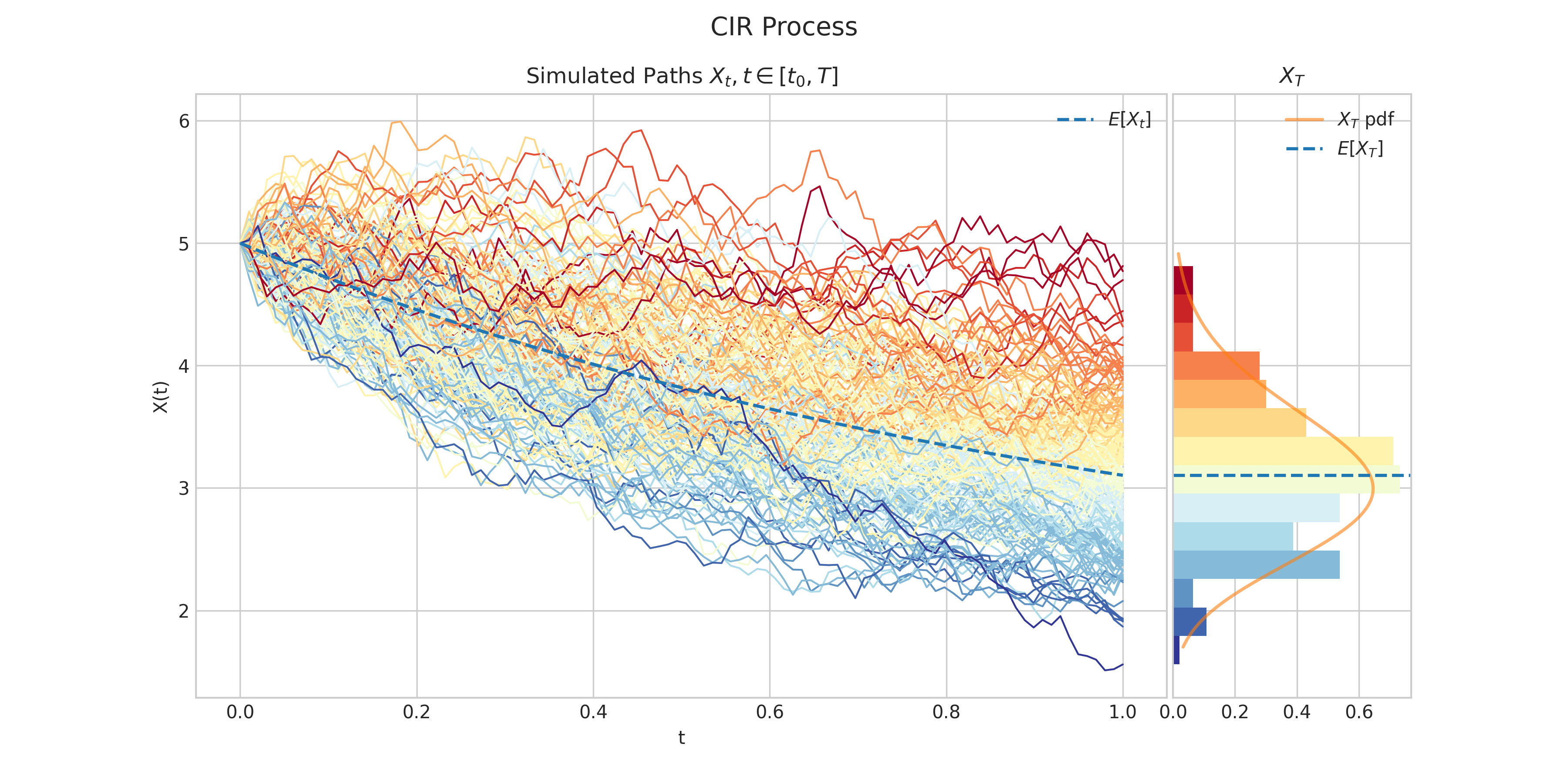
A Cox–Ingersoll–Ross process \(X = \{X : t \geq 0\}\) is characterised by the following Stochastic Differential Equation
\[dX_t = \theta(\mu - X_t) dt + \sigma \sqrt{X_t} dW_t, \ \ \ \ \forall t\in (0,T],\]with initial condition \(X_0 = x_0\), where
\(\theta\) is the rate of mean reversion
\(\mu\) is the long term mean value.
\(\sigma>0\) is the instantaneous volatility
\(W_t\) is a standard Brownian Motion.
Each \(X_t\) follows a non-central chi-square distribution.
- Parameters:
theta (float) – the parameter \(\theta\) in the above SDE
mu (float) – the parameter \(\mu\) in the above SDE
sigma (float) – the parameter \(\sigma>0\) in the above SDE
initial (float) – the initial condition \(x_0\) in the above SDE
T (float) – the right hand endpoint of the time interval \([0,T]\) for the process
rng (numpy.random.Generator) – a custom random number generator
- property T#
End time of the process.
- draw(n, N, marginal=True, envelope=False, title=None, **fig_kw)#
Simulates and plots paths/trajectories from the instanced stochastic process. Visualisation shows - times versus process values as lines - the expectation of the process across time - histogram showing the empirical marginal distribution \(X_T\) - probability density function of the marginal distribution \(X_T\) - envelope of confidence intervals
- Parameters:
n – number of steps in each path
N – number of paths to simulate
marginal – bool, default: True
envelope – bool, default: False
title – string optional default to None
- Returns:
- plot(n, N, title=None, **fig_kw)#
Simulates and plots paths/trajectories from the instanced stochastic process. Simple plot of times versus process values as lines and/or markers.
- Parameters:
n – number of steps in each path
N – number of paths to simulate
title – string to customise plot title
- Returns:
- simulate(n, N)#
Simulate paths/trajectories from the instanced stochastic process.
- Parameters:
n – number of steps in each path
N – number of paths to simulate
- Returns:
list with N paths (each one is a numpy array of size n)
- class aleatory.processes.CEVProcess(gamma=1.5, mu=0.5, sigma=0.1, initial=1.0, T=1.0, rng=None)[source]#
CEV or constant elasticity of variance process
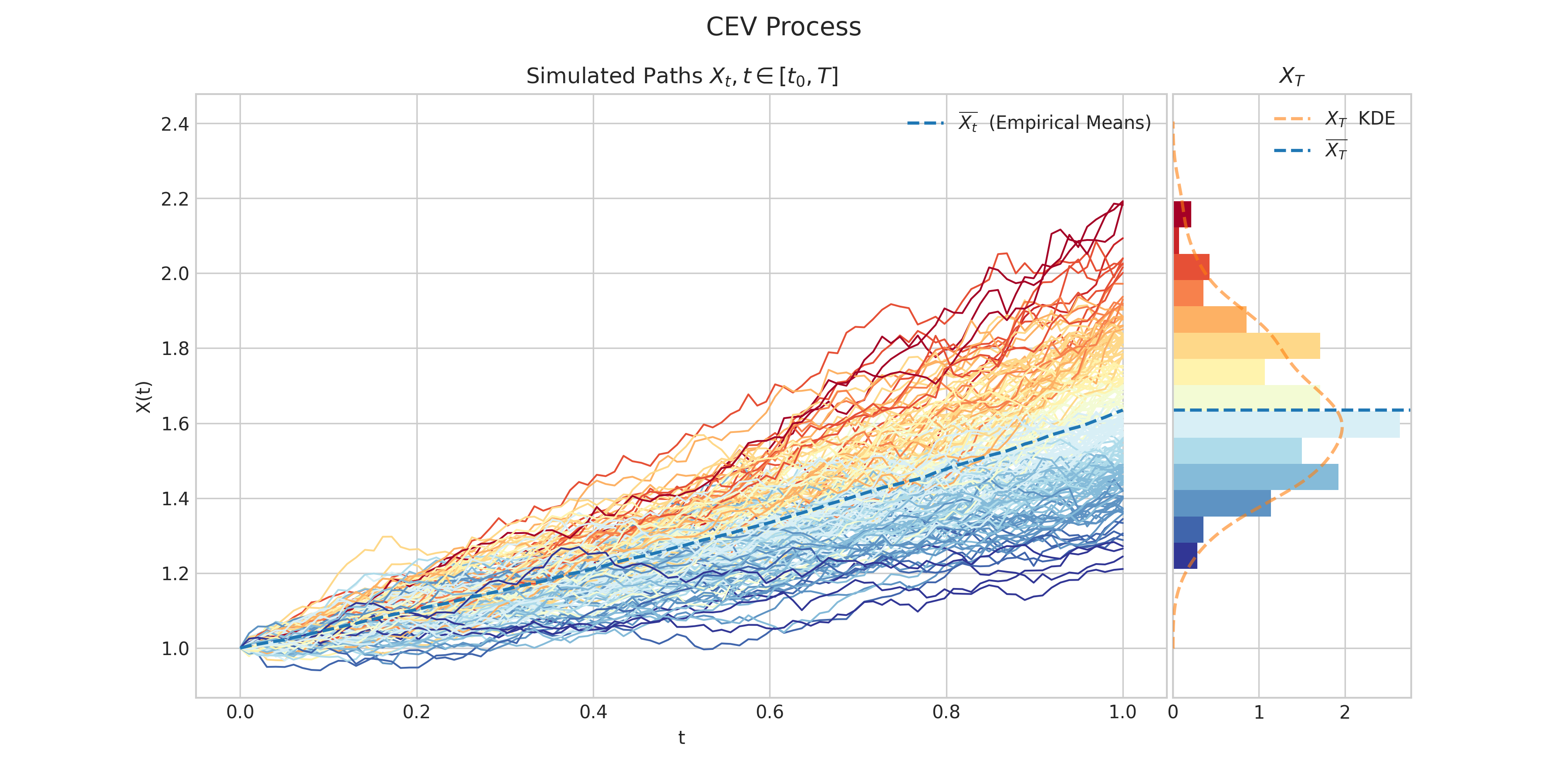
A CEV process \(X = \{X : t \geq 0\}\) is characterised by the following Stochastic Differential Equation
\[dX_t = \mu X_t dt + \sigma X_t^{\gamma} dW_t, \ \ \ \ \forall t\in (0,T],\]with initial condition \(X_0 = x_0\), where
\(\mu\) is the drift
\(\sigma>0\) is the scale of the volatility
\(\gamma\geq 0\) is the elasticity term
\(W_t\) is a standard Brownian Motion.
- Parameters:
mu (float) – the parameter \(\mu\) in the above SDE
sigma (float) – the parameter \(\sigma>0\) in the above SDE
gamma (float) – the parameter \(\gamma\) in the above SDE
initial (float) – the initial condition \(x_0\) in the above SDE
T (float) – the right hand endpoint of the time interval \([0,T]\) for the process
rng (numpy.random.Generator) – a custom random number generator
- property T#
End time of the process.
- draw(n, N, marginal=True, envelope=False, title=None, **fig_kw)[source]#
Simulates and plots paths/trajectories from the instanced stochastic process. Visualisation shows - times versus process values as lines - the expectation of the process across time - histogram showing the empirical marginal distribution \(X_T\) - probability density function of the marginal distribution \(X_T\) - envelope of confidence intervals
- Parameters:
n – number of steps in each path
N – number of paths to simulate
marginal – bool, default: True
envelope – bool, default: False
title – string optional default to None
- Returns:
- plot(n, N, title=None, **fig_kw)#
Simulates and plots paths/trajectories from the instanced stochastic process. Simple plot of times versus process values as lines and/or markers.
- Parameters:
n – number of steps in each path
N – number of paths to simulate
title – string to customise plot title
- Returns:
- simulate(n, N)#
Simulate paths/trajectories from the instanced stochastic process.
- Parameters:
n – number of steps in each path
N – number of paths to simulate
- Returns:
list with N paths (each one is a numpy array of size n)